Rate Distortion Theory

Note

We use \(p\) to denote fixed probability distributions, and \(q\) to denote probability distributions that are optimized.

Rate-distortion theory [CT06] is a framework for studying optimal lossy compression. Given a distribution \(p(x)\), we wish to find \(q(\hat{x}|x)\) which compresses \(X\) as much as possible while limiting the amount of user-defined distortion, \(d(x, \hat{x})\). The minimum rate (effectively, code book size) at which \(X\) can be compressed while maintaining a fixed distortion is known as the rate-distortion curve:

\[R(D) = \min_{q(\hat{x}|x), \langle d(x, \hat{x}) \rangle = D} \I{X : \hat{X}}\]

By introducing a Lagrange multiplier, we can transform this constrained optimization into an unconstrained one:

\[\mathcal{L} = \I{X : \hat{X}} + \beta \langle d(x, \hat{x}) \rangle\]

where minimizing at each \(\beta\) produces a point on the curve.

Example

It is known that under the Hamming distortion (\(d(x, \hat{x}) = \left[ x \neq \hat{x} \right]\)) the rate-distortion function for a biased coin has the following solution: \(R(D) = \H{p} - \H{D}\):

In [1]: In [1]: from dit.rate_distortion import RDCurve

Information Bottleneck

The information bottleneck [TPB00] is a form of rate-distortion where the distortion measure is given by:

\[d(x, \hat{x}) = D\left[~p(Y | x)~\mid\mid~q(Y | \hat{x})~\right]\]

where \(D\) is an arbitrary divergence measure, and \(\hat{X} - X - Y\) form a Markov chain. Traditionally, \(D\) is the Kullback-Leibler Divergence, in which case the average distortion takes a particular form:

\[\begin{split}\langle d(x, \hat{x}) \rangle &= \sum_{x, \hat{x}} q(x, \hat{x}) \DKL{ p(Y | x) || q(Y | \hat{x}) } \\ &= \sum_{x, \hat{x}} q(x, \hat{x}) \sum_{y} p(y | x) \log_2 \frac{p(y | x)}{q(y | \hat{x})} \\ &= \sum_{x, \hat{x}, y} q(x, \hat{x}, y) \log_2 \frac{p(y | x) p(x) p(y) q(\hat{x})}{q(y | \hat{x}) p(x) p(y) q(\hat{x})} \\ &= \sum_{x, \hat{x}, y} q(x, \hat{x}, y) \log_2 \frac{p(y | x) p(x)}{p(x) p(y)} \frac{p(y)q(\hat{x})}{q(y | \hat{x}) q(\hat{x})} \\ &= \I{X : Y} - \I{\hat{X} : Y}\end{split}\]

Since \(\I{X : Y}\) is constant over \(q(\hat{x} | x)\), it can be removed from the optimization. Furthermore,

\[\begin{split}\I{X : Y} - \I{\hat{X} : Y} &= (\I{X : Y | \hat{X}} + \I{X : Y : \hat{X}}) - (\I{Y : \hat{X} | X} + \I{X : Y : \hat{X}}) \\ &= \I{X : Y | \hat{X}} - \I{Y : \hat{X} | X} \\ &= \I{X : Y | \hat{X}}\end{split}\]

where the final equality is due to the Markov chain. Due to all this, Information Bottleneck utilizes a “relevance” term, \(\I{\hat{X} : Y}\), which replaces the average distortion in the Lagrangian:

\[\mathcal{L} = \I{X : \hat{X}} - \beta \I{\hat{X} : Y} ~.\]

Though \(\I{X : Y | \hat{X}}\) is the most simplified form of the average distortion, it is faster to compute \(\I{\hat{X} : Y}\) during optimization.

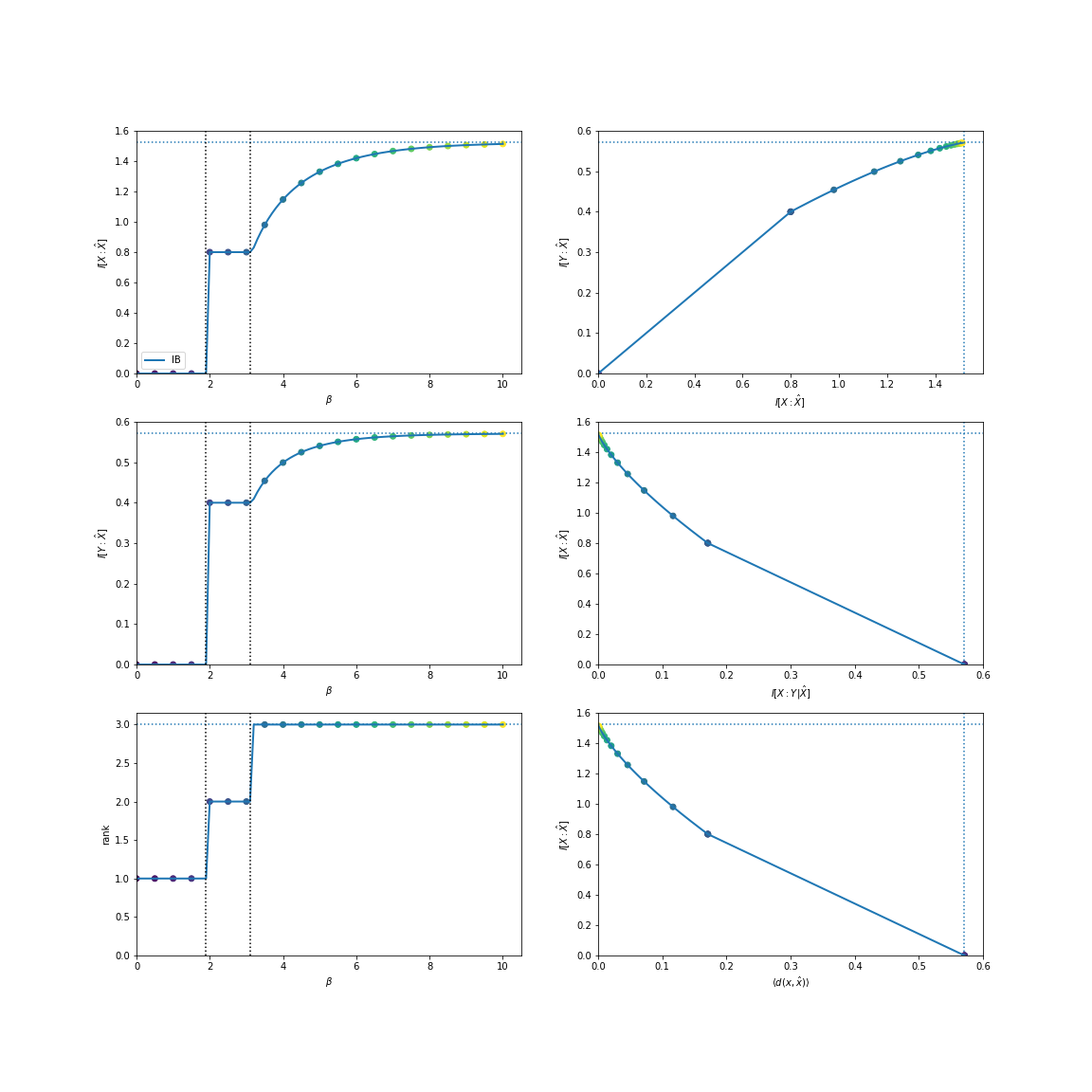
Example

Consider this distribution:

In [2]: In [4]: d = dit.Distribution(['00', '02', '12', '21', '22'], [1/5]*5)

There are effectively three features that the fist index, \(X\), has regarding the second index, \(Y\). We can find them using the standard information bottleneck:

In [3]: In [5]: from dit.rate_distortion import IBCurve

We can also find them utilizing the total variation:

In [4]: In [7]: from dit.divergences.pmf import variational_distance

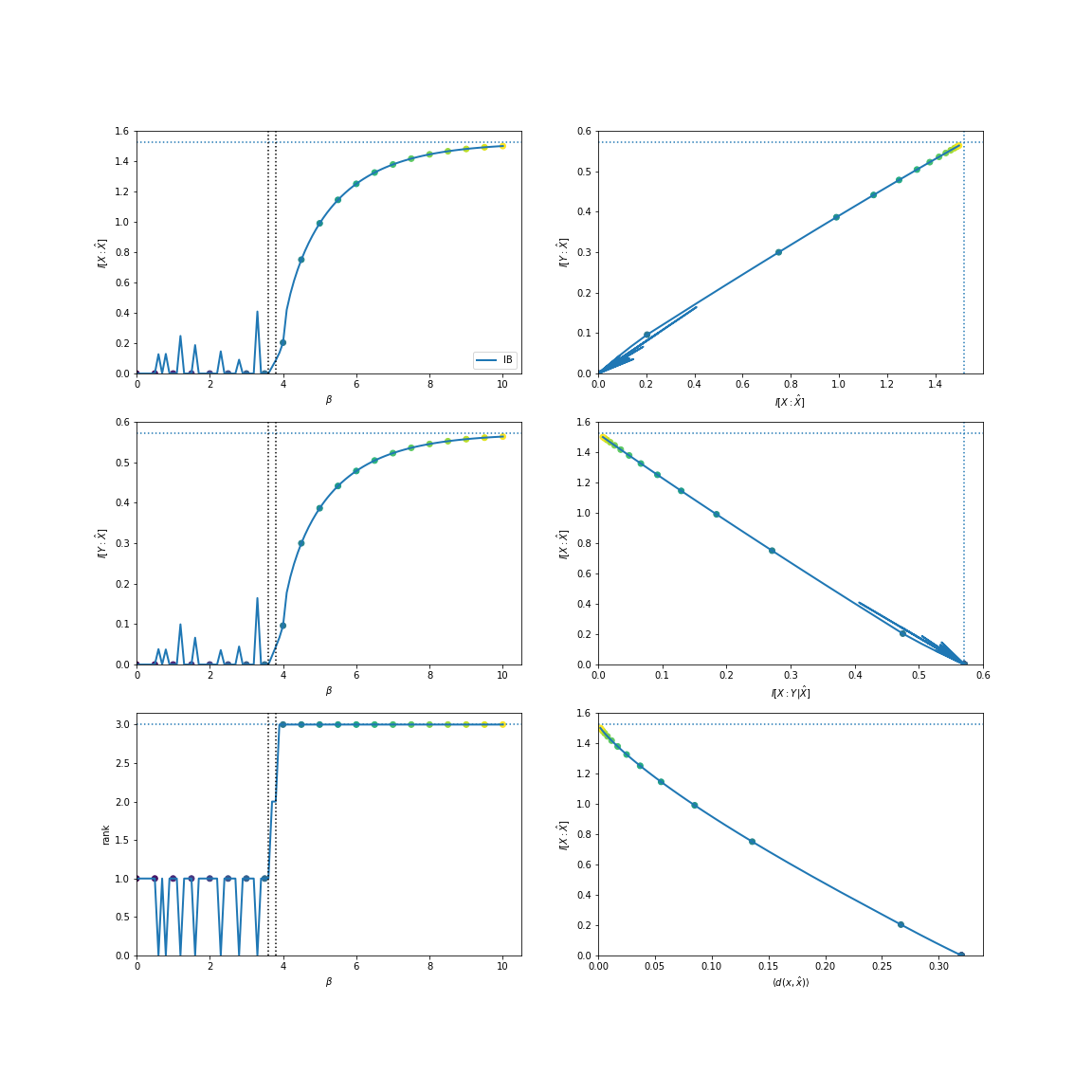
Note

The spiky behavior at low \(\beta\) values is due to numerical imprecision.

APIs

class RDCurve(dist, rv=None, crvs=None, beta_min=0, beta_max=10, beta_num=101, alpha=1.0, distortion=Distortion(name='Hamming', matrix=<function hamming_distortion>, optimizer=<class 'dit.rate_distortion.rate_distortion.RateDistortionHamming'>), method=None)

Compute a rate-distortion curve.

class IBCurve(dist, rvs=None, crvs=None, rv_mode=None, beta_min=0.0, beta_max=15.0, beta_num=101, alpha=1.0, method='sp', divergence=None)

Compute an information bottleneck curve.