Rate Distortion Theory

Note

We use \(p\) to denote fixed probability distributions, and \(q\) to denote probability distributions that are optimized.

Rate-distortion theory [CT06] is a framework for studying optimal lossy compression. Given a distribution \(p(x)\), we wish to find \(q(\hat{x}|x)\) which compresses \(X\) as much as possible while limiting the amount of user-defined distortion, \(d(x, \hat{x})\). The minimum rate (effectively, code book size) at which \(X\) can be compressed while maintaining a fixed distortion is known as the rate-distortion curve:

\[R(D) = \min_{q(\hat{x}|x), \langle d(x, \hat{x}) \rangle = D} \I{X : \hat{X}}\]

By introducing a Lagrange multiplier, we can transform this constrained optimization into an unconstrained one:

\[\mathcal{L} = \I{X : \hat{X}} + \beta \langle d(x, \hat{x}) \rangle\]

where minimizing at each \(\beta\) produces a point on the curve.

RDCurve minimizes \(\mathcal{L}\) with the Blahut-Arimoto algorithm [Ari72, Bla72], which alternates \(q(\hat{x}|x) \propto q(\hat{x}) 2^{-\beta d(x, \hat{x})}\) with \(q(\hat{x}) = \sum_x p(x) q(\hat{x}|x)\) (see also [CT06], Section 10.8). When the distortion does not depend on \(q\) (as for the Hamming distortion) the problem is convex, so two deterministic starts suffice, and the iteration stops once Blahut’s upper and lower bounds on \(\min \mathcal{L}\) agree. With \(c(x) = \sum_{\hat{x}} q(\hat{x}) 2^{-\beta d(x, \hat{x})}\), those bounds differ by \(\log_2 \max_{\hat{x}} \sum_x p(x) 2^{-\beta d(x, \hat{x})} / c(x)\). Distortions that depend on \(q\) (residual entropy, the information bottleneck) are not convex and keep multiple random restarts.

Example

It is known that under the Hamming distortion (\(d(x, \hat{x}) = \left[ x \neq \hat{x} \right]\)) the rate-distortion function for a biased coin has the following solution: \(R(D) = \H{p} - \H{D}\):

In [1]: from dit.rate_distortion import RDCurve

In [2]: d = dit.Distribution(['0', '1'], [1/2, 1/2])

In [3]: RDCurve(d, beta_num=26).plot();

Distortion Measures

RDCurve takes its distortion through the distortion argument. Three are provided in dit.rate_distortion:

• hamming (the default): \(d(x, \hat{x}) = \left[ x \neq \hat{x} \right]\).

• residual_entropy: \(d(x, \hat{x}) = -\log_2 q(x | \hat{x}) - \log_2 q(\hat{x} | x)\), whose average is the residual entropy of \(X\hat{X}\).

• maximum_correlation: penalizes the maximum correlation between \(X\) and \(\hat{X}\).

Each is a named tuple of a display name, a distortion matrix (when one exists), and the optimizer class that handles it. Note that the hamming distortion here is unrelated to the Hamming code dit.coding.hamming().

from dit.rate_distortion import RDCurve, residual_entropy

RDCurve(d, distortion=residual_entropy)

Information Bottleneck

The information bottleneck [TPB00] is a form of rate-distortion where the distortion measure is given by:

\[d(x, \hat{x}) = D\left[~p(Y | x)~\mid\mid~q(Y | \hat{x})~\right]\]

where \(D\) is an arbitrary divergence measure, and \(\hat{X} - X - Y\) form a Markov chain. Traditionally, \(D\) is the Kullback-Leibler Divergence, in which case the average distortion takes a particular form:

\[\begin{split}\langle d(x, \hat{x}) \rangle &= \sum_{x, \hat{x}} q(x, \hat{x}) \DKL{ p(Y | x) || q(Y | \hat{x}) } \\ &= \sum_{x, \hat{x}} q(x, \hat{x}) \sum_{y} p(y | x) \log_2 \frac{p(y | x)}{q(y | \hat{x})} \\ &= \sum_{x, \hat{x}, y} q(x, \hat{x}, y) \log_2 \frac{p(y | x) p(x) p(y) q(\hat{x})}{q(y | \hat{x}) p(x) p(y) q(\hat{x})} \\ &= \sum_{x, \hat{x}, y} q(x, \hat{x}, y) \log_2 \frac{p(y | x) p(x)}{p(x) p(y)} \frac{p(y)q(\hat{x})}{q(y | \hat{x}) q(\hat{x})} \\ &= \I{X : Y} - \I{\hat{X} : Y}\end{split}\]

Since \(\I{X : Y}\) is constant over \(q(\hat{x} | x)\), it can be removed from the optimization. Furthermore,

\[\begin{split}\I{X : Y} - \I{\hat{X} : Y} &= (\I{X : Y | \hat{X}} + \I{X : Y : \hat{X}}) - (\I{Y : \hat{X} | X} + \I{X : Y : \hat{X}}) \\ &= \I{X : Y | \hat{X}} - \I{Y : \hat{X} | X} \\ &= \I{X : Y | \hat{X}}\end{split}\]

where the final equality is due to the Markov chain. Due to all this, Information Bottleneck utilizes a “relevance” term, \(\I{\hat{X} : Y}\), which replaces the average distortion in the Lagrangian:

\[\mathcal{L} = \I{X : \hat{X}} - \beta \I{\hat{X} : Y} ~.\]

Though \(\I{X : Y | \hat{X}}\) is the most simplified form of the average distortion, it is faster to compute \(\I{\hat{X} : Y}\) during optimization.

Variants and Algorithms

The standard information bottleneck uses \(\I{X : \hat{X}}\) as the compression term. The generalized information bottleneck replaces this with

\[\H{\hat{X}} - \alpha \H{\hat{X} | X}\]

so that \(\alpha = 1\) recovers the standard bottleneck, while \(\alpha = 0\) gives the deterministic information bottleneck [SS16]. The deterministic endpoint minimizes

\[\H{\hat{X}} - \beta \I{\hat{X} : Y}\]

up to the constant \(\beta\I{X : Y}\), and its optima are hard clusterings of \(X\).

IBCurve supports these variants through variant='ib', variant='gib', and variant='dib'. The legacy alpha argument is still accepted: alpha=1 is standard IB, alpha=0 is DIB, and intermediate values are generalized IB. The default method='sp' uses the generic optimizer. method='ba' uses the Blahut-Arimoto-style finite-alphabet iteration for the standard, unconditional IB. method='sequential' and method='agglomerative' use finite-alphabet hard-clustering algorithms for the unconditional DIB; the latter follows the information-based clustering viewpoint of building a hierarchy by merging clusters [SATkavcikB05].

For deterministic prediction tasks, where \(Y\) is a function of \(X\), sweeps over the IB Lagrangian can miss portions of the IB curve and can include trivial solutions. Interpret kinks and beta sweeps in those cases with care [KTVK18].

Example

Consider this distribution:

In [4]: d = dit.Distribution(['00', '02', '12', '21', '22'], [1/5]*5)

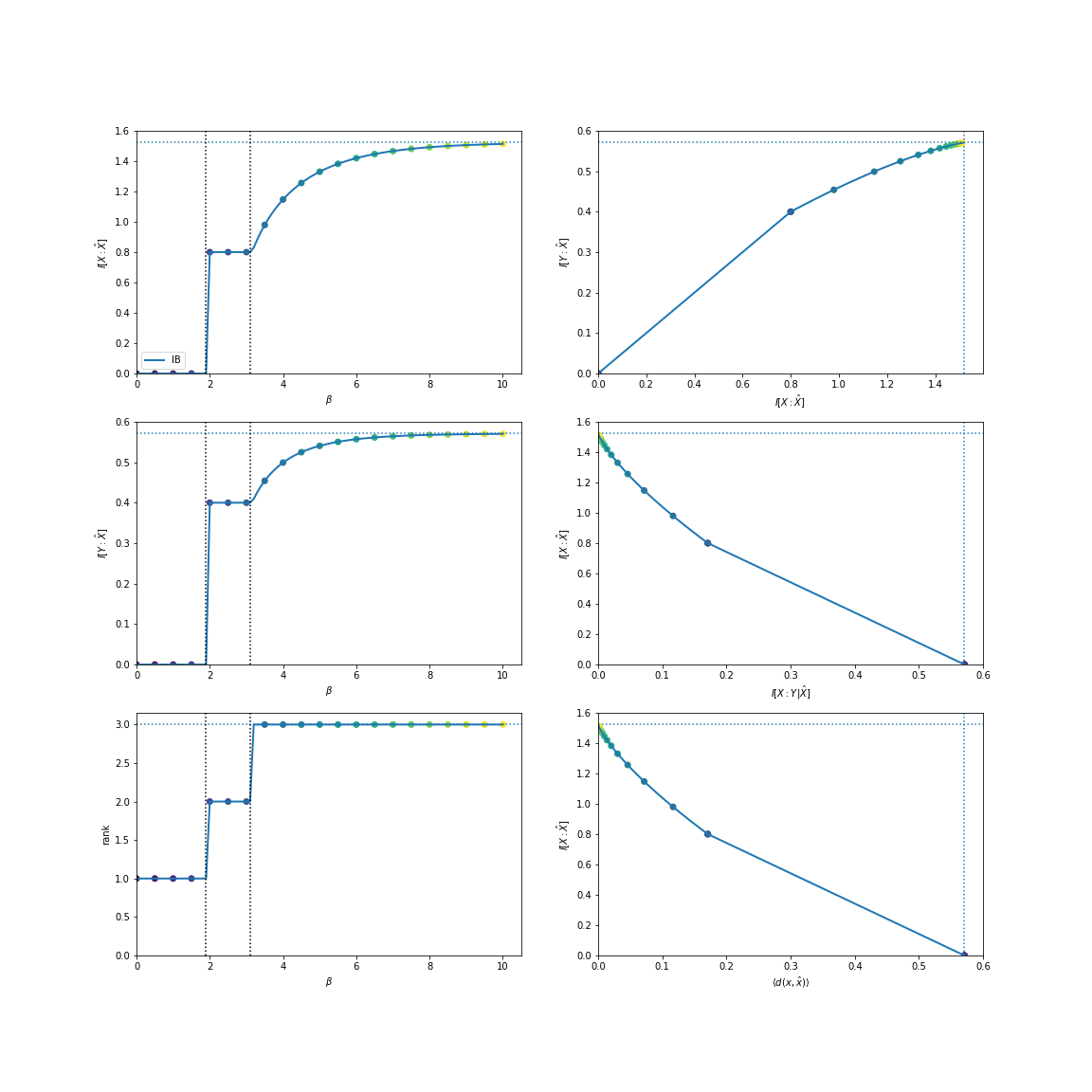
There are effectively three features that the first index, \(X\), has regarding the second index, \(Y\). We can find them using the standard information bottleneck:

In [5]: from dit.rate_distortion import IBCurve

In [6]: IBCurve(d, beta_num=26).plot();

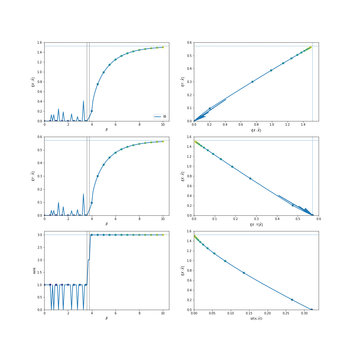
We can also find them utilizing the total variation:

In [7]: from dit.divergences.pmf import variational_distance

In [8]: IBCurve(d, divergence=variational_distance).plot();

Note

The spiky behavior at low \(\beta\) values is due to numerical imprecision.

Passing divergence makes IBCurve use InformationBottleneckDivergence, the bottleneck whose distortion is \(D[p(Y | x) \mid\mid q(Y | \hat{x})]\) for an arbitrary divergence \(D\) operating on probability vectors (see dit.divergences.pmf).

The deterministic information bottleneck can be computed with a hard-clustering solver:

In [9]: IBCurve(d, variant='dib', method='sequential', beta_num=26).plot();

Privacy Funnel

The privacy funnel [MSFMedard14] is the information bottleneck turned around. Given private data \(S\) and public data \(X\), we release \(T\), a randomized function of \(X\) (so that \(S - X - T\) form a Markov chain), which is informative about \(X\) but reveals as little as possible about \(S\):

\[\mathrm{PF}(R) = \min_{q(t|x), \I{X : T} \geq R} \I{S : T}\]

The leakage \(\I{S : T}\) and utility \(\I{X : T}\) are both convex in \(q(t|x)\), so their difference is not, and the privacy funnel is a non-convex problem. Its Lagrangian is

\[\mathcal{L} = \I{S : T} - \beta \I{X : T}\]

Since \(\I{S : T} \leq \I{X : T}\), every \(\beta \geq 1\) is minimized by releasing \(T = X\), so the Lagrangian is swept over \(\beta \in [0, 1]\).

For a fixed \(p(s, x)\), the pairs \((\I{X : T}, \I{S : T})\) over all releases \(T\) form a convex set. Its upper boundary is the information bottleneck curve of \(X\) with respect to \(S\), and its lower boundary is the privacy funnel curve [AC20]. So the privacy funnel curve is convex and increasing. Since it often has a narrow range of slopes, a sweep over \(\beta\) resolves few of its points, and PFCurve sweeps the rate \(R\) instead. The size of \(T\) is bounded by \(|X| + 1\); unlike the information bottleneck, \(|X|\) does not suffice in general [AC20].

greedy_privacy_funnel implements the greedy algorithm of [MSFMedard14]: starting from \(T = X\), it repeatedly merges the two symbols of \(T\) whose merger most reduces the leakage while the utility is at least \(R\). Each step is locally optimal, but the result need not be optimal overall.

Perfect Privacy

A release with non-zero utility and zero leakage exists if and only if the vectors \(p(S | x)\) are linearly dependent [CMMedard15]; in particular, whenever \(|X| > |S|\). The largest utility of such a release,

\[g_0 = \max_{q(t|x), \I{S : T} = 0} \I{X : T}\]

is computed exactly by perfect_privacy_utility. Every such \(T\) writes \(p(X)\) as a mixture of distributions \(p(X | t)\) under which \(S\) is distributed as \(p(S)\). These form a polytope, and since entropy is concave, the optimal mixture uses only its vertices; the mixing weights then solve a linear program [RGunduz21].

Example

Let \(S\) be binary and \(X\) ternary:

In [10]: from dit.rate_distortion import admits_perfect_privacy, perfect_privacy_utility, privacy_funnel_rate

In [11]: d = dit.Distribution(['00', '01', '12', '10'], [0.3, 0.2, 0.3, 0.2])

In [12]: admits_perfect_privacy(d)
Out[12]: True

In [13]: perfect_privacy_utility(d)
Out[13]: 0.6954618442383221

In [14]: privacy_funnel_rate(d, 1.2)
Out[14]: 0.22904935197227727

BottleneckRegionPlotter computes both curves and plots the region between them:

In [15]: from dit.rate_distortion.plotting import BottleneckRegionPlotter

In [16]: BottleneckRegionPlotter.from_dist(d).plot();

See Also

The The Gray-Wyner Network extends rate-distortion ideas to a one-encoder, many-decoder network, and recovers the common informations as operating points.

APIs

class RDCurve(dist, rv=None, crvs=None, beta_min=0, beta_max=10, beta_num=101, alpha=1.0, distortion=('Hamming', <function hamming_distortion>, <class 'dit.rate_distortion.rate_distortion.RateDistortionHamming'>), method=None)

Compute a rate-distortion curve.

class IBCurve(dist, rvs=None, crvs=None, beta_min=0.0, beta_max=15.0, beta_num=101, alpha=1.0, method='sp', divergence=None, variant=None, bound=None)

Compute an information bottleneck curve.

class InformationBottleneck(dist, beta, alpha=1.0, rvs=None, crvs=None, bound=None)

Base optimizer for information bottleneck type calculations.

class GeneralizedInformationBottleneck(dist, beta, alpha=1.0, rvs=None, crvs=None, bound=None)

The generalized information bottleneck family.

The parameter alpha interpolates between the standard information bottleneck (alpha=1) and the deterministic information bottleneck (alpha=0).

class DeterministicInformationBottleneck(dist, beta, alpha=0.0, rvs=None, crvs=None, bound=None)

The deterministic information bottleneck objective.

This is the alpha=0 endpoint of the generalized information bottleneck, using \(H(T | Z)\) as the compression term.

class InformationBottleneckDivergence(dist, beta, alpha=1.0, divergence=<function relative_entropy_pmf>, rvs=None, crvs=None, bound=None)

A generalized information bottleneck which uses a distortion equal to D( p(Y|x) || q(Y|t) ) for an arbitrary divergence measure D.

class PFCurve(dist, rvs=None, crvs=None, rate_num=26, method='sp', bound=None)

Compute a privacy funnel curve [MSFMedard14]: the least leakage I[S : T | Z] of a release T of X as a function of its utility I[X : T | Z]. It is the lower boundary of the region whose upper boundary is the information bottleneck curve of X with respect to S [AC20].

The curve is swept over utility rates rather than Lagrange multipliers: it is convex, often with a narrow range of slopes, so a sweep over the multiplier would resolve only a few of its points.

class PrivacyFunnel(dist, beta, rvs=None, crvs=None, bound=None)

The privacy funnel Lagrangian [MSFMedard14],

\[\min_{p(t | x, z)} I[S : T | Z] - \beta I[X : T | Z],\]

over mappings T of X, so that S - XZ - T. Since I[S : T | Z] <= I[X : T | Z], every beta >= 1 is minimized by releasing T = X, so the whole curve is traced by beta in [0, 1]. The objective is a difference of convex functions of the mapping, so it is non-convex [AC20].

class PrivacyFunnelRate(dist, rate, rvs=None, crvs=None, bound=None)

The privacy funnel [MSFMedard14],

\[\mathrm{PF}(R) = \min_{p(t | x, z) : I[X : T | Z] \geq R} I[S : T | Z].\]

The size of T is bounded by |X| + 1; unlike the information bottleneck, |X| does not suffice in general [AC20].

privacy_funnel(dist, beta, rvs=None, crvs=None, bound=None)

Compute a point on the privacy funnel by minimizing I[S : T | Z] - beta I[X : T | Z] [MSFMedard14].

Parameters:

• dist (Distribution) – The distribution of interest.

• beta (float) – The non-negative price of utility.

• rvs (iterable of iterables, None) – The private variables S and the public variables X. If None, use dist.rvs.

• crvs (iterable, None) – The random variables to condition on.

• bound (int, None) – The bound on the size of T. If None, use |X|.

Returns:

• leakage (float) – I[S : T | Z] at the optimum.

• utility (float) – I[X : T | Z] at the optimum.

privacy_funnel_rate(dist, rate, rvs=None, crvs=None, bound=None)

Compute the privacy funnel, the least leakage I[S : T | Z] of a release T of X with utility I[X : T | Z] >= rate [MSFMedard14].

Parameters:

• dist (Distribution) – The distribution of interest.

• rate (float) – The minimum utility, in bits.

• rvs (iterable of iterables, None) – The private variables S and the public variables X. If None, use dist.rvs.

• crvs (iterable, None) – The random variables to condition on.

• bound (int, None) – The bound on the size of T. If None, use |X| + 1.

Returns:

pf – The minimal leakage.

Return type:

float

greedy_privacy_funnel(p_sx, rate=0.0)

Greedily merge released symbols for the privacy funnel [MSFMedard14].

Starting from \(T = X\), repeatedly merge the pair of symbols of \(T\) whose merger most reduces the leakage \(I(S : T)\) while keeping the utility \(I(X : T) \geq R\), until no merge is feasible. Each step is locally optimal; the result need not be globally optimal.

Parameters:

• p_sx (np.ndarray) – Joint distribution with axis 0 indexing the private \(S\) and axis 1 indexing the public \(X\).

• rate (float) – The minimum utility \(R\), in bits. Must lie in \([0, H(X)]\).

Returns:

result – The hard privacy mapping found.

Return type:

PrivacyFunnelResult

Raises:

ditException – If rate is outside \([0, H(X)]\).

class PrivacyFunnelResult(p_t_given_x: ndarray, leakage: float, utility: float, active: int, assignments: ndarray | None = None, merges: tuple[tuple[int, int], ...] = ())

The result of a finite-alphabet privacy funnel optimization.

p_t_given_x

The privacy mapping \(p(t | x)\).

Type:

np.ndarray

leakage

\(I(S : T)\).

Type:

float

utility

\(I(X : T)\).

Type:

float

active

The number of non-empty released states.

Type:

int

assignments

The hard cluster assignment for each \(x\), when available.

Type:

np.ndarray

merges

The merge sequence, when available.

Type:

tuple[tuple[int, int], …]

admits_perfect_privacy(dist, rvs=None)

Determine whether X can be released with non-zero utility and zero leakage about S.

This is the case if and only if the vectors p(S | x), over the support of X, are linearly dependent [CMMedard15]; in particular, whenever |X| > |S|.

Parameters:

• dist (Distribution) – The distribution of interest.

• rvs (iterable of iterables, None) – The private variables S and the public variables X. If None, use dist.rvs.

Returns:

perfect – Whether perfect privacy is possible.

Return type:

bool

perfect_privacy_utility(dist, rvs=None, return_mechanism=False, max_candidates=100000)

Compute the maximal utility at perfect privacy,

\[g_0 = \max_{p(t | x) : I(S : T) = 0} I(X : T),\]

exactly, by enumerating the vertices of the perfect privacy polytope and solving a linear program [RGunduz21].

Parameters:

• dist (Distribution) – The distribution of interest.

• rvs (iterable of iterables, None) – The private variables S and the public variables X. If None, use dist.rvs.

• return_mechanism (bool) – If True, also return an optimal mapping p(t | x).

• max_candidates (int) – The maximum number of column bases to enumerate.

Returns:

• g0 (float) – The maximal utility, in bits, of a release leaking nothing about S.

• p_t_given_x (np.ndarray) – An optimal mapping of shape (|X|, |T|), if return_mechanism.

Raises:

ditException – If the polytope has too many candidate bases.

class BottleneckRegionPlotter(ib_curve=None, pf_curve=None)

Plot the information bottleneck and privacy funnel curves together. For a fixed p(s, x), every release T of X gives a point (I[X : T | Z], I[S : T | Z]); these points form a convex region whose upper boundary is the information bottleneck curve and whose lower boundary is the privacy funnel curve [AC20].

classmethod from_dist(dist, rvs=None, crvs=None, ib_kwargs=None, pf_kwargs=None)

Compute both curves of a distribution and build a plotter for them.

Parameters:

• dist (Distribution) – The distribution of interest.

• rvs (iterable, None) – The private variables S and the public variables X. If None, use [0], [1].

• crvs (iterable, None) – The random variables to condition on.

• ib_kwargs (dict, None) – Extra keyword arguments for IBCurve.

• pf_kwargs (dict, None) – Extra keyword arguments for PFCurve.

Returns:

plotter – The plotter.

Return type:

BottleneckRegionPlotter

plot(ax=None, num=201)

Plot the region.

Parameters:

• ax (mpl.Axis, None) – The axis to plot on. If None, make a new figure.

• num (int) – The number of points used to shade the region.

Returns:

fig – The figure containing the plot.

Return type:

mpl.Figure